Introduction

Cluster analysis or clustering is the task of grouping a set of objects in such a way that objects in the same group (called cluster) are more similar (in some sense or another) to each other than to those in other groups (clusters).

Clustering can be applied to microarray data to identify groups of possibly co-regulated genes or spatial gene expression patterns.

In Anja von Heydebreck’s presentation Clustering analysis for microarray data, he introduced many clustring methods including K-means clusting, PAM and Hierarchical clustering. He also gave some R packages which implemented these jobs. I will try to summary cluster analysis methods in R using microarray datasets.

Sample Data

The bioconductor project has various packages for experimental data. To install bioconductor packages, a special tool called biocLite is used. The demo data Golub is installed with the following command in R.

source("http://bioconductor.org/biocLite.R")
biocLite("golubEsets")

The Golub et al. (1999) data consist of 47 patients with acute lymphoblastic leukemia (ALL) and 25 patients with acute myeloid leukemia (AML). Each of the 72 patients had bone marrow samples obtained at the time of diagnosis. Furthermore, the observations have been assayed with Affymetrix Hgu6800 chips, resulting in 7129 gene expressions (Affymetrix probes).

As discussed in the Bioconductor manual, “ALL arises from two different types of lymphocytes (T-cell and B-cell)”, so we may wish to consider the data in terms of three classes: AML, ALL-T, and ALL-B. We provide the option to consider the data as two or three classes. Also, the Golub data set is often seen in two forms. In one case, the data are partitioned into a training and a test data set: we provide these as Golub_Train and Golub_Test, respectively. In the other case, the training and the test data sets are combined into one data set: we have named this golub.

The Golub data set is possibly the most widely studied and cited microarray data set.

# load require package and datasets
library(golubEsets)
data(Golub_Merge)
golub <- data.frame(Golub_Merge)[1:7129]
# calculate variance and rearrange columns by variance decreasingly
golub.rearrange <- golub[ , order(apply(golub, 2, var), decreasing=T)]
golub <- golub.rearrange[, 1:150]

Then golub is the new dataset for use with all the following clustering methods.

Partitioning

The partitioning methods generally result in a set of M clusters, each object belonging to one cluster. Each cluster may be represented by a centroid or a cluster representative. If the number of the clusters is large, the centroids can be further clustered to produces hierarchy within a dataset.

K-means Clustering

R supports K-means Clustering by default. The kmeans() function can be used to do this and 4 algorithms are available. When using K-means Clustering, the number of clusters should be determined in advance. Here we set the number of clusters to be 8.

# K-Means Cluster Analysis
fit <- kmeans(x=golub, 8)

Result is stored in an S3 object of class “kmeans”. Information like cluster assignment and cluster centers can be extracted using the following commands.

fit$cluster  # get cluster assignment
fit$centers  # get cluster center
# get cluster means
aggregate(golub, by=list(fit$cluster), FUN=mean)

Partitioning Around Medoids

K-means clustering is based on Euclidean distance. PAM generalizes the idea and can be used with any distance measure. Just as in K-means clustering, PAM requires the number of clusters to be determined in advance. R recommands the cluster package (installed with R) for PAM. It implemented a pam object and summary methods.

require(cluster) 
fit <- pam(x=golub, k=8)

The assignment and the medoids are still of interest.

fit$clustering # get cluster assignment
fit$medoids # get coordinates of each medoid
# summary method
summary(fit)

Hierarchical Agglomerative

Hierarchical Clustering is a method of cluster analysis which seeks to build a hierarchy of clusters. Agglomerative is a “bottom up” approach: each observation starts in its own cluster, and pairs of clusters are merged as one moves up the hierarchy. R also supports it by default in hclust(), with the distance matrix can be calculated using one of “euclidean”, “maximum”, “manhattan”, “canberra”, “binary” or “minkowski” distance.

# Ward Hierarchical Clustering
d <- dist(golub, method = "euclidean") # distance matrix
fit <- hclust(d, method="ward") 

## The "ward" method has been renamed to "ward.D"; note new "ward.D2"

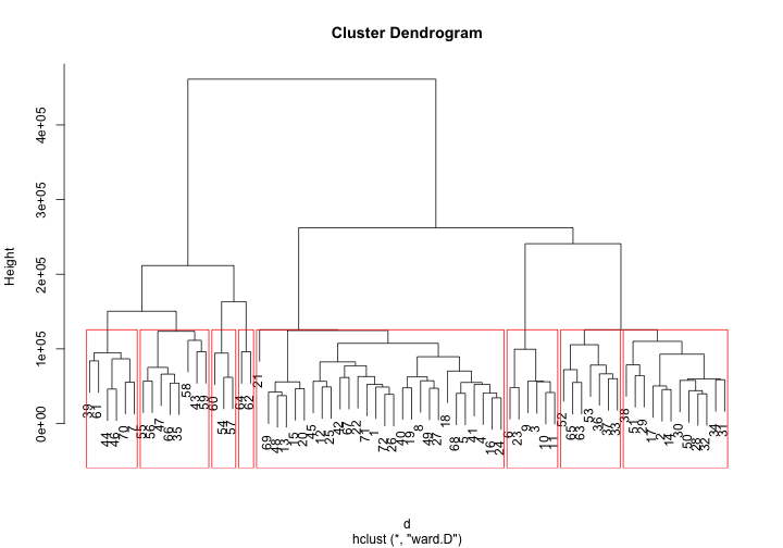
Hierarchical Clustering will be better understood in plots. R has special plot methods for plotting an object of class hclust.

plot(fit)
groups <- cutree(fit, k=8) # cut tree into 5 clusters
# draw dendogram with red borders around the 5 clusters 
rect.hclust(fit, k=8, border="red")

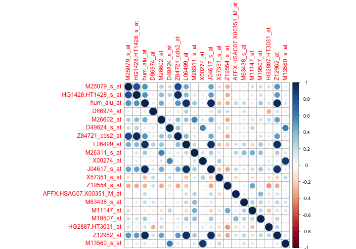
Visualization of Similarity

As Heydebreck mentioned that a direct visualization is more informative. It’s useful when one wants to investigate a specific factor. Here we just inspect the correlation of the genes with the highest variance.

library(corrplot)
corrplot(cor(golub.rearrange[ , 1:20]))

Conclusions

These are just basic some basic cluster analysis in R. R implemented several user-friendly functions to do cluster analysis. As you can see from the above example, R code are always simple and readable. Therefore, Clustering algorithms are easy to apply and they are useful for exploratory analysis.

(If you have trouble viewing this page, please download the pdf version.)